Python GEKKO ODE unexpected result

Python GEKKO ODE unexpected result … here is a solution to the problem.

Python GEKKO ODE unexpected result

I’ve been trying to implement ODE models to model the insulin signaling pathway, as shown in <a href=”https://www.jbc.org/article/S0021-9258(19)48589-X/fulltext#seccestitle10″ rel=”noreferrer noopener nofollow”>this paper , Use python’s GEKKO

The implemented model variant is “Md3” with the following equations, constants, and initial values:

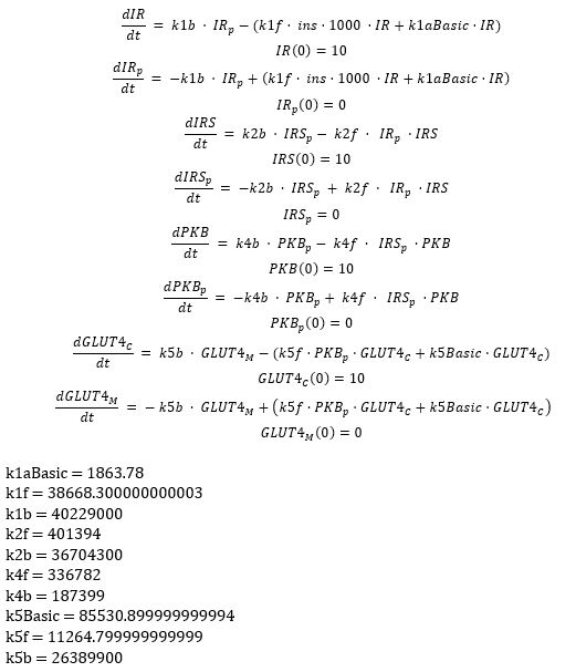
Even if this paper does not provide the result of the supplementary code, one would expect the result to be a curve, not the result produced by my code: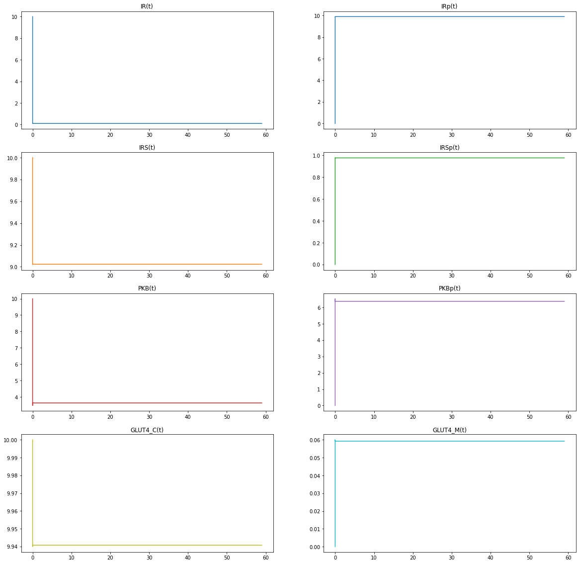

I’VE CHECKED EQUATIONS AND CONSTANT VALUES, TRIED ADDING LOWER AND UPPER BOUNDS FOR VARIABLES, AND TRIED USING THE M.OPTIONS.IMODE AND M.OPTIONS.NODES PARAMETERS, BUT THESE DON’T SEEM TO HELP.

Any suggestions would be appreciated.

def insulin_pathway_CM(time_interval, insulin=0): 

m = GEKKO()
    t = np.linspace(0, time_interval-1, time_interval)
    m.time = np.insert(t,1,[1e-5,1e-4,1e-3,1e-2,0.1])

# initialization of variables
    ins = m.Param(value=insulin)
    IR = m.Var(10)
    IRp = m.Var()
    IRS = m.Var(10)
    IRSp = m.Var()
    PKB = m.Var(10)
    PKBp = m.Var()
    GLUT4_C = m.Var(10)
    GLUT4_M = m.Var()
  
# initialization of constants                                                                                                                                                 
    k1aBasic = 1863.78                                                                   
    k1f = 38668.300000000003                                                             
    k1b = 40229000                                                                       
    k2f = 401394                                                                         
    k2b = 36704300                                                                       
    k4f = 336782                                                                         
    k4b = 187399  
    k5Basic = 85530.899999999994  
    k5f = 11264.799999999999 
    k5b = 26389900   

# equations
    m.Equation(IR.dt() == k1b*IRp - (k1f*ins*1000*IR + k1aBasic*IR))
    m.Equation(IRp.dt() == -k1b*IRp + k1f*ins*1000*IR + k1aBasic*IR)
    m.Equation(IRS.dt() == k2b*IRSp - (k2f*IRp*IRS))
    m.Equation(IRSp.dt() == -k2b*IRSp + k2f*IRp*IRS)
    m.Equation(PKB.dt() == k4b*PKBp - k4f*IRSp*PKB)
    m.Equation(PKBp.dt() == -k4b*PKBp + k4f*IRSp*PKB)
    m.Equation(GLUT4_C.dt() == k5b*GLUT4_M - (k5f*PKBp*GLUT4_C + k5Basic*GLUT4_C))
    m.Equation(GLUT4_M.dt() == -k5b*GLUT4_M + (k5f*PKBp*GLUT4_C + k5Basic*GLUT4_C))

m.options.IMODE = 7
    m.options.OTOL  = 1e-8
    m.options.RTOL  = 1e-8
    m.options.NODES = 3
    m.solve(disp=False)

# plotting
    fig, axs = plt.subplots(4, 2, figsize=(20, 20))
    axs[0, 0].plot(m.time, IR)
    axs[0, 0].set_title('IR(t)')
    axs[0, 1].plot(m.time, IRp)
    axs[0, 1].set_title('IRp(t)')
    axs[1, 0].plot(m.time, IRS, 'tab:orange')
    axs[1, 0].set_title('IRS(t)')
    axs[1, 1].plot(m.time, IRSp, 'tab:green')
    axs[1, 1].set_title('IRSp(t)')
    axs[2, 0].plot(m.time, PKB, 'tab:red')
    axs[2, 0].set_title('PKB(t)')
    axs[2, 1].plot(m.time, PKBp, 'tab:purple')
    axs[2, 1].set_title('PKBp(t)')
    axs[3, 0].plot(m.time, GLUT4_C, 'tab:olive')
    axs[3, 0].set_title('GLUT4_C(t)')
    axs[3, 1].plot(m.time, GLUT4_M, 'tab:cyan')
    axs[3, 1].set_title('GLUT4_M(t)')
    
plt.figure()
    plt.show()
    return

time_interval = 60
insulin = 100
insulin_pathway_CM(time_interval, insulin)

Solution

Lutz Lehmann is right. Derivative plots with end times of 1e-5 show that most of the action occurs over a short period of time.

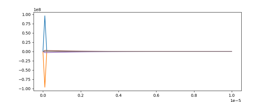
Try to shorten the time span.

m.time = np.linspace(0,1e-5,100)

This shows rapid dynamics.

There may be errors in the equation, such as a unit problem (time in days or years?). Or the author forgot to include some type of volume factor for the patient, such as blood volume or volume.

# equations
V1 = 1e9  # hypothetical volume 1
V2 = 10   # hypothetical volume 2
m.Equation(V1*IR.dt() == k1b*IRp - (k1f*ins*1000*IR + k1aBasic*IR))
m.Equation(V1*IRp.dt() == -k1b*IRp + k1f*ins*1000*IR + k1aBasic*IR)
m.Equation(V1*IRS.dt() == k2b*IRSp - (k2f*IRp*IRS))
m.Equation(V1*IRSp.dt() == -k2b*IRSp + k2f*IRp*IRS)
m.Equation(V2*PKB.dt() == k4b*PKBp - k4f*IRSp*PKB)
m.Equation(V2*PKBp.dt() == -k4b*PKBp + k4f*IRSp*PKB)
m.Equation(V2*GLUT4_C.dt() == k5b*GLUT4_M - (k5f*PKBp*GLUT4_C + k5Basic*GLUT4_C))
m.Equation(V2*GLUT4_M.dt() == -k5b*GLUT4_M + (k5f*PKBp*GLUT4_C + k5Basic*GLUT4_C))

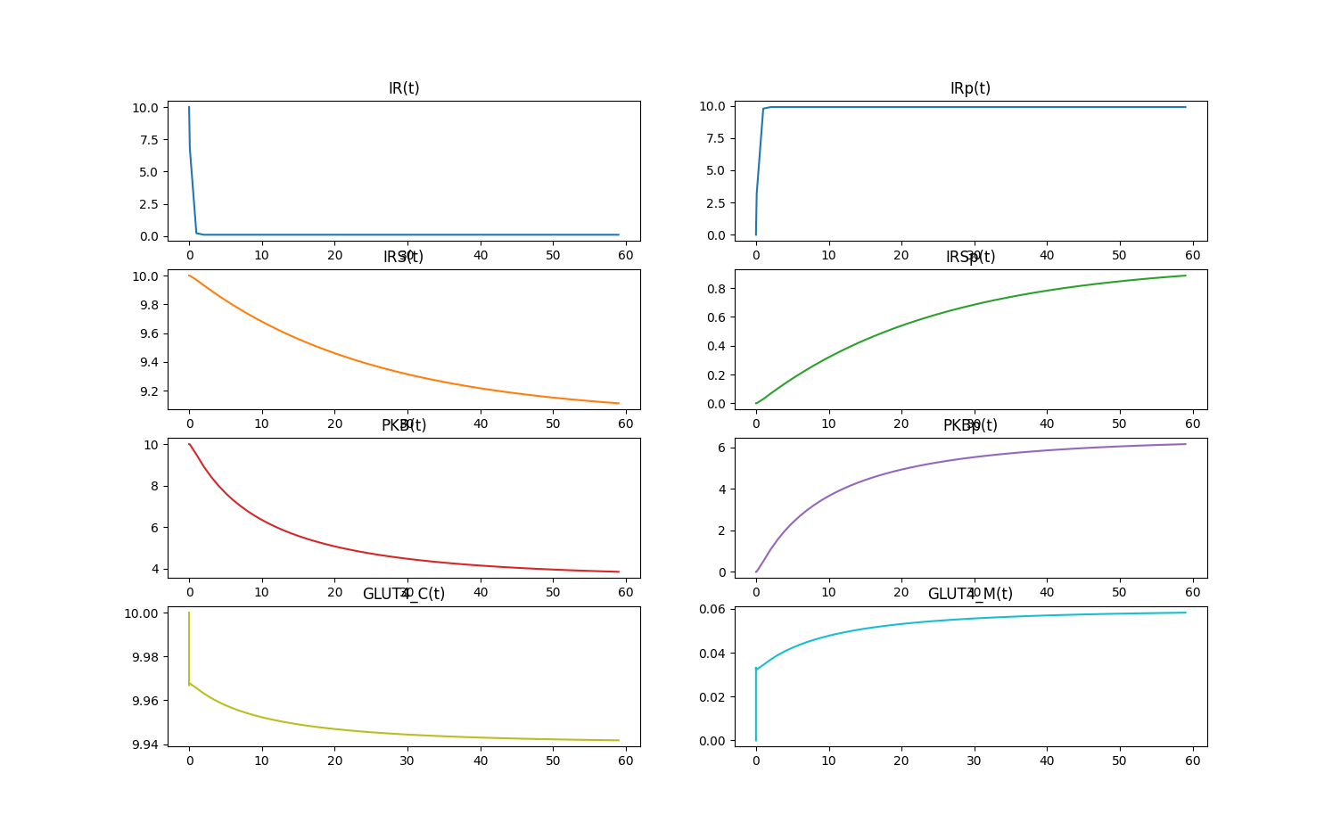
Here are more plausible dynamics on the original timescale (0-60 hours).

from gekko import GEKKO
import numpy as np
import matplotlib.pyplot as plt

def insulin_pathway_CM(time_interval, insulin=0): 

m = GEKKO()
    t = np.linspace(0, time_interval-1, time_interval)
    m.time = np.insert(t,1,[1e-5,1e-4,1e-3,1e-2,0.1])

# initialization of variables
    ins = m.Param(value=insulin)
    IR = m.Var(10)
    IRp = m.Var()
    IRS = m.Var(10)
    IRSp = m.Var()
    PKB = m.Var(10)
    PKBp = m.Var()
    GLUT4_C = m.Var(10)
    GLUT4_M = m.Var()
  
# initialization of constants
    k1aBasic = 1863.78      
    k1f = 38668.300000000003  
    k1b = 40229000  
    k2f = 401394 
    k2b = 36704300 
    k4f = 336782
    k4b = 187399  
    k5Basic = 85530.899999999994  
    k5f = 11264.799999999999 
    k5b = 26389900   

# calculate derivatives
    d = m.Array(m.Var,8)
    m.Equation(d[0] == k1b*IRp - (k1f*ins*1000*IR + k1aBasic*IR))
    m.Equation(d[1] == -k1b*IRp + k1f*ins*1000*IR + k1aBasic*IR)
    m.Equation(d[2] == k2b*IRSp - (k2f*IRp*IRS))
    m.Equation(d[3] == -k2b*IRSp + k2f*IRp*IRS)
    m.Equation(d[4] == k4b*PKBp - k4f*IRSp*PKB)
    m.Equation(d[5] == -k4b*PKBp + k4f*IRSp*PKB)
    m.Equation(d[6] == k5b*GLUT4_M - (k5f*PKBp*GLUT4_C + k5Basic*GLUT4_C))
    m.Equation(d[7] == -k5b*GLUT4_M + (k5f*PKBp*GLUT4_C + k5Basic*GLUT4_C))    

# equations
    V1 = 1e9  # hypothetical volume 1
    V2 = 10   # hypothetical volume 2
    m.Equation(V1*IR.dt() == k1b*IRp - (k1f*ins*1000*IR + k1aBasic*IR))
    m.Equation(V1*IRp.dt() == -k1b*IRp + k1f*ins*1000*IR + k1aBasic*IR)
    m.Equation(V1*IRS.dt() == k2b*IRSp - (k2f*IRp*IRS))
    m.Equation(V1*IRSp.dt() == -k2b*IRSp + k2f*IRp*IRS)
    m.Equation(V2*PKB.dt() == k4b*PKBp - k4f*IRSp*PKB)
    m.Equation(V2*PKBp.dt() == -k4b*PKBp + k4f*IRSp*PKB)
    m.Equation(V2*GLUT4_C.dt() == k5b*GLUT4_M - (k5f*PKBp*GLUT4_C + k5Basic*GLUT4_C))
    m.Equation(V2*GLUT4_M.dt() == -k5b*GLUT4_M + (k5f*PKBp*GLUT4_C + k5Basic*GLUT4_C))

m.options.IMODE = 4
    m.options.OTOL  = 1e-8
    m.options.RTOL  = 1e-8
    m.options.NODES = 3
    m.solve(disp=True)

# plotting
    fig, axs = plt.subplots(4, 2, figsize=(20, 20))
    axs[0, 0].plot(m.time, IR)
    axs[0, 0].set_title('IR(t)')
    axs[0, 1].plot(m.time, IRp)
    axs[0, 1].set_title('IRp(t)')
    axs[1, 0].plot(m.time, IRS, 'tab:orange')
    axs[1, 0].set_title('IRS(t)')
    axs[1, 1].plot(m.time, IRSp, 'tab:green')
    axs[1, 1].set_title('IRSp(t)')
    axs[2, 0].plot(m.time, PKB, 'tab:red')
    axs[2, 0].set_title('PKB(t)')
    axs[2, 1].plot(m.time, PKBp, 'tab:purple')
    axs[2, 1].set_title('PKBp(t)')
    axs[3, 0].plot(m.time, GLUT4_C, 'tab:olive')
    axs[3, 0].set_title('GLUT4_C(t)')
    axs[3, 1].plot(m.time, GLUT4_M, 'tab:cyan')
    axs[3, 1].set_title('GLUT4_M(t)')

plt.figure()
    for i in range(8):
        plt.plot(m.time,d[i].value)
    
plt.show()
    return

time_interval = 60
insulin = 100
insulin_pathway_CM(time_interval, insulin)

As a reference, here’s a simplified blood glucose response model (similar to the Bergman model) for everyone to quote. Richard Bergman and Claudio Cobelli proposed a minimal model describing blood glucose and insulin dynamics in 1979.

Python GEKKO ODE unexpected result

Solution

Related Problems and Solutions