Python – How to use basemap to map the field of view of Earth observation satellites near the poles?

I am trying to map the maximum (theoretical) view of the satellite along its orbit. I’m using a basemap, I want to plot different locations along the track (scatter plot) on it, and I want to add the entire field of view using the tissot method (or equivalent).
In a 300 km high-altitude orbit, before about 75 degrees north latitude, the code below works fine. Beyond this code outputs ValueError:
“ValueError: Undefined geodesic (possibly enantidote)

”

import matplotlib.pyplot as plt
from mpl_toolkits.basemap import Basemap
import math

earth_radius = 6371000.  # m
fig = plt.figure(figsize=(8, 6), edgecolor='w')
m = Basemap(projection='cyl', resolution='l',
            llcrnrlat=-90, urcrnrlat=90,
            llcrnrlon=-180, urcrnrlon=180)

# draw the coastlines on the empty map
m.drawcoastlines(color='k')

# define the position of the satellite
position = [300000., 75., 0.]  # altitude, latitude, longitude

# radius needed by the tissot method
radius = math.degrees(math.acos(earth_radius / (earth_radius + position[0])))
m.tissot(position[2], position[1], radius, 100, facecolor='tab:blue', alpha=0.3)
m.scatter(position[2], position[1], marker='*', c='tab:red')

plt.show()

Notice that the code works fine at the South Pole (latitude below -75). I know this is a known bug, is there a known workaround for this issue?
Thanks for your help!

What you find are some limitations of Basemap. Let’s switch to Cartopy for now. The working code will be different, but not much.

import matplotlib.pyplot as plt
import cartopy.crs as ccrs
import math

earth_radius = 6371000.
position = [300000., 75., 0.]   # altitude (m), lat, long
radius = math.degrees(math.acos(earth_radius / (earth_radius + position[0])))
print(radius)  # in subtended degrees??

fig = plt.figure(figsize=(12,8))

img_extent = [-180, 180, -90, 90]

# here, cartopy's' `PlateCarree` is equivalent with Basemap's `cyl` you use
ax = fig.add_subplot(1, 1, 1, projection = ccrs. PlateCarree(), extent = img_extent)

# for demo purposes, ...
# let's take 1 subtended degree = 112 km on earth surface (*** you set the value as needed ***)
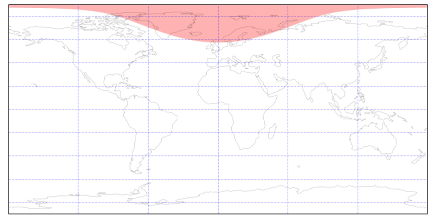
ax.tissot(rad_km=radius*112, lons=position[2], lats=position[1], n_samples=64, \
             facecolor='red', edgecolor='black', linewidth=0.15, alpha = 0.3)

ax.coastlines(linewidth=0.15)
ax.gridlines(draw_labels=False, linewidth=1, color='blue', alpha=0.3, linestyle='--')
plt.show()

Using the code above, the resulting graph is:

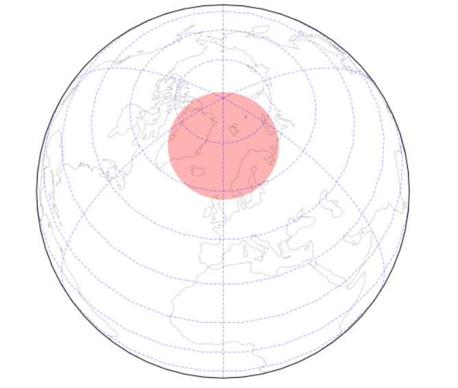
Now, if we use orthogonal projection, (replace the relevant line of code with this).

ax = fig.add_subplot(1, 1, 1, projection = ccrs. Orthographic(central_longitude=0.0, central_latitude=60.0))

You get this plot: