Python – Plot 4D data as hierarchical heat maps in Python

I want to use (x,y,z) coordinates and a color-based fourth dimension to create a layered heat map to correlate with intensity.

The data associated with each layer is in a text file that contains columns x, y, z, and g. The delimiter is a space. We apologize if it is displayed incorrectly.

XA
200
600
1200
1800
2400
3000
200
600
1200
1800
2400
3000

Yes.
0
0
0
0
0
0
600
600
600
600
600
600

ZA
600
600
600
600
600
600
600
600
600
600
600
600

Genetic algorithm
1.27
1.54
1.49
1.34
1.27
1.25
1.28
1.96
1.12
1.06
1.06
1.06

import numpy as np
import matplotlib.pyplot as plt
from mpl_toolkits.mplot3d import Axes3D

data = np.load(filename)

x = np.linspace(0,2400,num=6)
y = np.linspace(0,2400,num=11)
X,Y=np.meshgrid(x,y)
Z = data[:,:,0] * 1e-3

plt.contourf(X,Y,Z)
plt.colorbar()

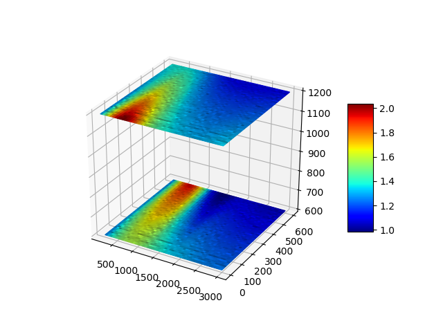
How do I read a text file, create and overlay a heat map along the Z axis?

Let’s say you have two txt files, data-z600.txt and data-z1200.txt, in the same folder as your python script with exactly the same contents

Data-Z600.txt (yours).

XA YA ZA GA
200 0 600 1.27
600 0 600 1.54
1200 0 600 1.49
1800 0 600 1.34
2400 0 600 1.27
3000 0 600 1.25
200 600 600 1.28
600 600 600 1.96
1200 600 600 1.12
1800 600 600 1.06
2400 600 600 1.06
3000 600 600 1.06

and Data-Z1200.txt (intentionally invented).

XA YA ZA GA
200 0 1200 1.31
600 0 1200 2
1200 0 1200 1.63
1800 0 1200 1.36
2400 0 1200 1.31
3000 0 1200 1.35
200 600 1200 1.38
600 600 1200 1.36
1200 600 1200 1.2
1800 600 1200 1.1
2400 600 1200 1.1
3000 600 1200 1.11

Let’s import all the required libraries

# libraries
from mpl_toolkits.mplot3d import Axes3D
import matplotlib.pyplot as plt
import scipy.interpolate as si
from matplotlib import cm
import pandas as pd
import numpy as np

and define grids_maker, which is a function that prepares the data contained in a given file, here via the filepath parameter.

def grids_maker(filepath):
    # Get the data
    df = pd.read_csv(filepath, sep=' ')

# Make things more legible
    xy = df[['XA', 'YA']]
    x  = xy. XA
    y  = xy. YA
    z  = df. ZA
    g  = df. GA
    reso_x = reso_y = 50
    interp = 'cubic' # or 'nearest' or 'linear'

# Convert the 4d-space's dimensions into grids
    grid_x, grid_y = np.mgrid[
        x.min():x.max():1j*reso_x,
        y.min():y.max():1j*reso_y
    ]

grid_z = si.griddata(
        xy, z.values,
        (grid_x, grid_y),
        method=interp
    )

grid_g = si.griddata(
        xy, g.values,
        (grid_x, grid_y),
        method=interp
    )

return {
        'x' : grid_x,
        'y' : grid_y,
        'z' : grid_z,
        'g' : grid_g,
    }

Let’s use grids_maker for our list of files and get the extremum of the 4th dimension for each file.

# Let's retrieve all files' contents
fgrids = dict.fromkeys([
    'data-z600.txt',
    'data-z1200.txt'
])
g_mins = []
g_maxs = []

for fpath in fgrids.keys():
    fgrids[fpath] = grids = grids_maker(fpath)
    g_mins.append(grids['g'].min())
    g_maxs.append(grids['g'].max())

Let’s create our (uniform for all files) color scale

# Create the 4th color-rendered dimension
scam = plt.cm.ScalarMappable(
    norm=cm.colors.Normalize(min(g_mins), max(g_maxs)),
    cmap='jet' # see https://matplotlib.org/examples/color/colormaps_reference.html
)

… Finally, produce/show the plot

# Make the plot
fig = plt.figure()
ax  = fig.gca(projection='3d')
for grids in fgrids.values(): 
    scam.set_array([])   
    ax.plot_surface(
        grids['x'], grids['y'], grids['z'],
        facecolors  = scam.to_rgba(grids['g']),
        antialiased = True,
        rstride=1, cstride=1, alpha=None
    )
plt.show()