Python – An interactive satellite map that uses Python

I’m trying to overlay Lambert Conformal Conical satellite imagery onto a Holoviews interactive map. I can map satellite images well, but I can’t figure out how to properly translate this map onto the Holoviews map. Below is my reproducible code for getting data using the Unidata Siphon library.

Import the package

from datetime import datetime
import matplotlib.pyplot as plt
from netCDF4 import Dataset
from siphon.catalog import TDSCatalog
import holoviews as hv
import geoviews as gv
import geoviews.feature as gf
from cartopy import crs
from cartopy import feature as cf

hv.extension('bokeh')

Get the data and create the graph

date=datetime.utcnow()
idx=-2
regionstr = 'CONUS'
channelnum = 13
datestr = str(date.year) + "%02d"%date.month + "%02d"%date.day
channelstr = 'Channel' + "%02d"%channelnum

cat = TDSCatalog('http://thredds-test.unidata.ucar.edu/thredds/catalog/satellite/goes16/GOES16/' + regionstr +
    '/' + channelstr + '/' + datestr + '/catalog.xml')
ds = cat.datasets[idx].remote_access(service='OPENDAP')
x = ds.variables['x'][:]
y = ds.variables['y'][:]
z = ds.variables['Sectorized_CMI'][:]

proj_var = ds.variables[ds.variables['Sectorized_CMI'].grid_mapping]

# Create a Globe specifying a spherical earth with the correct radius
globe = ccrs. Globe(ellipse='sphere', semimajor_axis=proj_var.semi_major,
                   semiminor_axis=proj_var.semi_minor)

proj = ccrs. LambertConformal(central_longitude=proj_var.longitude_of_central_meridian,
                             central_latitude=proj_var.latitude_of_projection_origin,
                             standard_parallels=[proj_var.standard_parallel],
                             globe=globe)

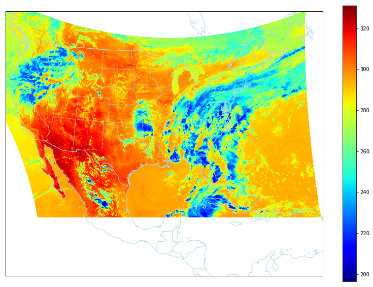
fig = plt.figure(figsize=(14, 10))
ax = fig.add_subplot(1, 1, 1, projection=proj)
ax.coastlines(resolution='50m', color='lightblue')
ax.add_feature(cf. STATES, linestyle=':', edgecolor='lightblue')
ax.add_feature(cf. BORDERS, linewidth=1, edgecolor='lightblue')

for im in ax.images:
    im.remove()
im = ax.imshow(z, extent=(x.min(), x.max(), y.min(), y.max()), origin='upper', cmap='jet')
plt.colorbar(im)

Now use Holoviews (using the Bokeh backend) to draw interactive images

goes = hv. Dataset((x, y, z),['Lat', 'Lon'], 'ABI13')
%opts Image (cmap='jet') [width=1000 height=800 xaxis='bottom' yaxis='left' colorbar=True toolbar='above' projection=proj] 
goes.to.image()* gf.coastline().options(projection=crs. LambertConformal(central_longitude=proj_var.longitude_of_central_meridian,central_latitude=proj_var.latitude_of_projection_origin,standard_parallels=[proj_ var.standard_parallel],globe=globe))

I

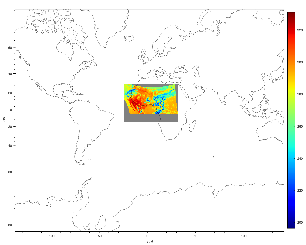
must not have translated it correctly, although I found very little documentation on Holoviews about Lambert’s conformal conic projection. I’m willing to use any other interactive map package. My main wish is to be able to draw relatively quickly, get state/country lines correctly on the image, and be able to zoom in. I’ve tried folium but also ran into projection issues.

So I think the main thing is to understand, that is, to explain here: how the forecast was announced. Elements in GeoViews, such as images, points, and so on, have a parameter called crs, which declares the coordinate system in which the data resides, and the projection drawing option declares what to project for the displayed data.

In your case, I guess you want to display the image in the same coordinate system it already has (Lambert Conformal), so technically you don’t have to declare a coordinate system (crs) on the element, you can just use hv. Image (completely unaware of the projection).

As far as I know, if you’re using GeoViews 1.5, your code should already work as expected, but I’ll do it :

# Apply mask
masked = np.ma.filled(z, np. NaN)

# Declare image from data
goes = hv. Image((x, y, masked),['Lat', 'Lon'], 'ABI13')

# Declare some options
options = dict(width=1000, height=800, yaxis='left', colorbar=True,
               toolbar='above', cmap='jet', projection=proj)

# Display plot
gf.ocean * gf.land * goes.options(**options) * gf.coastline.options(show_bounds=False)

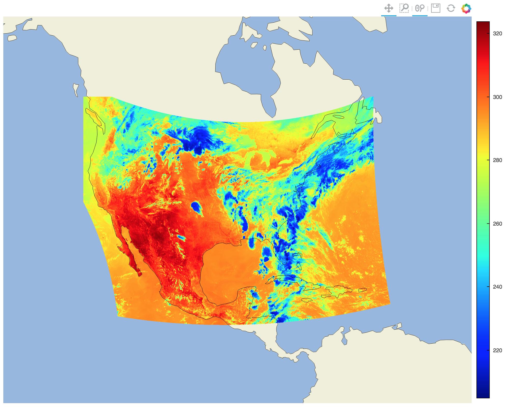
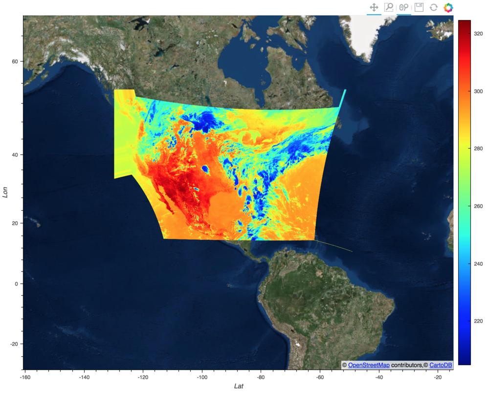
Notice how we declare projections on Image, not crs. If you really want to display the data in different projections that define it, you must declare a crs and use gv. Image。 In this case, I recommend using an project_image with the fast option enabled (this may introduce some artifacts, but it’s a lot of speed):

# Apply mask
masked = np.ma.filled(z, np. NaN)

# Declare the gv. Image with the crs
goes = gv. Image((x, y, masked), ['Lat', 'Lon'], 'ABI13', crs=proj)

# Now regrid the data and apply the reprojection
projected_goes = gv.operation.project_image(goes, fast=False, projection=ccrs. GOOGLE_MERCATOR)

# Declare some options
options = dict(width=1000, height=800, yaxis='left', colorbar=True,
               toolbar='above', cmap='jet')

# Display plot
projected_goes.options(**options) * gv.tile_sources. ESRI.options(show_bounds=False)

Another final tip, when you draw with Bokeh, all the data you’re drawing will be sent to the browser, so when working with larger images than you’re already using, I recommend using HoloViews’ regrid action, which uses data shaders to dynamically resize the image when zoomed. To use it, just apply the action to the image like this:

from holoviews.operation.datashader import regrid
regridded = regrid(goes)